![]() Matlab - Calcul sur les polynômes
Matlab - Calcul sur les polynômes
![]()
2- Détermination des coefficients d’un polynôme à partir des ses racines
4- Fractions rationnelles : Décomposition en éléments simples
conv |
produit de polynômes |
residue | décomposition
en éléments simples |
roots | trouve
les racines d'un polynôme |
poly | trouve
le polynôme à partir des ses racines |
polyval
| évalue
le polynôme |
3x² - 5x + 2 = 0
On commence par définir un " vecteur " qui contient les coefficients du polynôme :
>> p = [ 3 -5 2 ]
p =
3 -5 2
>> roots(p)
ans =
1.0000
0.6667
>> roots( [ 3 -5 2 ])
ans =
1.0000
0.6667
x² - 4x + 4 = 0
>> p= [ 1 -4 4 ]
p =
1 -4 4
>> roots(p)
ans =
2
2
x² + 3x + 8 = 0
>> p= [ 1 3 8 ]
p =
1 3 8
>> roots(p)
ans =
-1.5000 + 2.3979i
-1.5000 - 2.3979i
![]()
>> p = [ 1 2 -2 4 3 5 ]
p =
1 2 -2 4 3 5
>> roots(p)
ans =
-3.0417
0.9704 + 1.0983i
0.9704 - 1.0983i
-0.4495 + 0.7505i
-0.4495 - 0.7505i
>> format long e
>> roots(p)
ans =
-3.041684725314715e+000
9.703604093970790e-001 +1.098343294996758e+000i
9.703604093970790e-001 -1.098343294996758e+000i
-4.495180467397220e-001 +7.504870344729816e-001i
-4.495180467397220e-001 -7.504870344729816e-001i
polynôme à coefficients complexes :
(1+i)x² + (2-5i)x + 3,5 = 0
>> format short
>> p = [ 1+i 2-5i 3.5]
p =
1.0000 + 1.0000i 2.0000 - 5.0000i 3.5000
>> roots(p)
ans =
1.7116 + 4.0248i
-0.2116 - 0.5248i
2- Détermination des coefficients d’un polynôme à partir des ses racines
>> a = [ 2 1 ]
a =
2 1
>> poly(a)
ans =
1 -3 2
(c’est-à-dire : x² -3x +2)
>> a = [ 2 2 3 -5 ]
a =
2 2 3 -5
>> poly(a)
ans =
1 -2 -19 68 -60
>> a = [ 2+i 2-3i 5]
a =
2.0000 + 1.0000i 2.0000 - 3.0000i 5.0000
>> poly(a)
ans =
1.0000 -9.0000 + 2.0000i 27.0000 -14.0000i -35.0000 +20.0000i
Vérification :
>> p = ans
p =
1.0000 -9.0000 + 2.0000i 27.0000 -14.0000i -35.0000 +20.0000i
>> roots(p)
ans =
2.0000 - 3.0000i
5.0000 - 0.0000i
2.0000 + 1.0000i
( x –2 )( x – 1 ) = ?
>> p1=[ 1 -2 ]
p1 =
1 -2
>> p2=[ 1 -1 ]
p2 =
1 -1
>> conv( p1 , p2 )
ans =
1 -3 2
Autrement dit :
( x –2 )( x – 1 ) = x² -3x +2
(3x² - 5x + 2)( x² + 3x + 8) = ?
>> p1=[ 3 -5 2 ]
p1 =
3 -5 2
>> p2=[ 1 3 8 ]
p2 =
1 3 8
>> conv( p1 , p2 )
ans =
3 4 11 -34 16
Autrement écrit :
(3x² - 5x + 2)( x² + 3x + 8) = 3x4 + 4x3 + 11 x² -34 x +16
4- Décomposition en éléments simples
![]()
p1 , p2 … désignent les " pôles ".
![]()
polynôme du numérateur :
>> n =[ 6 ]
n =
6
polynôme du dénominateur :
>> d =[ 1 6 11 6 0 ]
d =
1 6 11 6 0
>> [ r , p , k ] = residue ( n , d)
r =
-1.0000
3.0000
-3.0000
1.0000
p =
-3.0000
-2.0000
-1.0000
0
k =
[ ]
Finalement :
![]()
y = f(x) = 3x² - 5x + 2
5-1- Utilisation de la fonction plot
>> p = [ 3 -5 2 ]
p =
3 -5 2
Calcul de f( x = 1) :
>> polyval( p , 1 )
ans =
0
Calcul de f( x = 2) :
>> polyval( p , 2)
ans =
4
Création du vecteur x :
>> x = 0 : 0.01 : 2
x =
Columns 1 through 7
0 0.0100 0.0200 0.0300 0.0400 0.0500 0.0600
…
Columns 197 through 201
1.9600 1.9700 1.9800 1.9900 2.0000
Création du vecteur y :
>> y = polyval( p , x)
y =
Columns 1 through 7
2.0000 1.9503 1.9012 1.8527 1.8048 1.7575 1.7108
…
Columns 197 through 201
3.7248 3.7927 3.8612 3.9303 4.0000
>> plot (x , y)
>> grid on
5-2- Utilisation de la fonction fplot
5-2-1- Première méthode
>> fplot ( '3*x^2 - 5*x + 2' , [ 0 2 ] )
>> grid on
5-2-2- Deuxième méthode
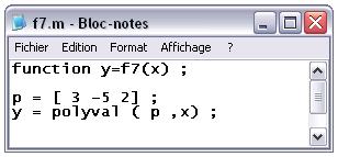
Il faut créer le fichier .m de la fonction :
>> f7(2)
ans =
4
>> f7(0)
ans =
2
>> fplot ('f7', [ 0 2] )
>> grid on
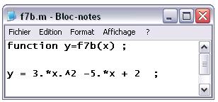
On peut également définir le polynôme de la manière suivante :
© Fabrice Sincère ; Révision 0.9.7